LLM Study Notes IV: Multimodal Large Language Models

VLM (Vision-Language Models)

VLMs exhibit a strong capability of both image and text understanding. A good use case is answering questions regarding the image. This would involve both spatial and semantic understanding of the image, with basic knowledge and reasoning abilities in text. The basic structure is taking embeddings from both image and text encoders and perform cross attention.

Pre-Training

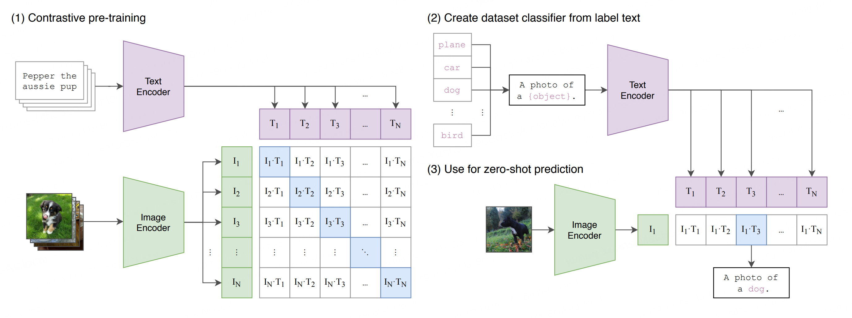
This is the contrastive learning part in CLIP, where massive dataset of image-text pairs are used to align image tokens with text tokens.

Fine-Tuning

The aligned tokens are then cross-attended and trained for specific downstream tasks, such as VQA, image-captioning, image-text retrieval, etc. The dataset used for fine-tuning is usually smaller but requires high quality, and sometimes synthetic data combined with bootstrapping methods are used (like in BLIP).

Vision Transformer (ViT)

It’s basically just a flattened language transformer.

First of all, the model overview. Vision transformer is encoder only:

The whole point is to flatten 2D image patches into 1D sequence of embeddings, and position embedding is still based on learnable 1D, since no significant improvement when using 2D-aware position embeddings. This linear projection of flattened patches is the tokenization of image patches, analogous to the tokenization of words in LLM, except for LLM it’s using a pre-defined token mapping, usually not through neural network.

The classification is similar to that of BERT, by prepending a class token at the front of the flattened embeddings, so we have \(z_0^0=\text{<CLS>}, z_0^1, ..., z_0^T\), and the final encoder output embeddings would be \(z_L^0=\mathbf{y}, z_L^1,...,z_L^T\). The length of output embedding sequence depends on the patch and image sizes.

There are two common ways to digest these embeddings:

1. Using just one pooled embedding \(\mathbf{y}\) only, where it goes through a linear head to get final prediction logit for classification. This is the main purpose in the original ViT paper. CLIP uses this \(\mathbf{y}\) embedding as the summary token for later text embedding alignment. Note that even though only token is explicitly used to generate classification tag, the bidirectional attention ensures the other padding embeddings are also well-encoded and contain meaningful information about the image.
2. Use the entire encoder output embeddings. This provides a much richer context with spatial information of the image for downstream task. For example,
   1. Masked Autoencoder (MAE) uses random masks on patches and their embeddings, and train the decoder to fill out these parts;
   2. DINO uses two ViTs, teacher and student, on same image with different augmentations, to align feature distributions for self-distillation, which is really strong on semantic grouping/clustering;
   3. Most VLMs such as BLIP use the full patch embeddings for cross-attention with text embeddings for tasks like caption generation and image QA.

ViT is the cornerstone of all multi-modal models. Depending on different type of tasks trained downstream, the pre-trained ViT encoders have different properties accordingly. Based on the model size and data scale, VLMs can choose whether to use frozen weights ViT, PEFT (usually LoRA), or full-fledge e2e training. Length of the embeddings depends on the patch and image sizes.

CLIP (Contrastive Language-Image Pre-Training)

The figure in original CLIP paper illustrates its contrastive training nature perfectly. The output embeddings of text encoder and ViT encoder are individually projected into a joint multi-modal embedding space:

A similarity function is then measured across each image and text embedding pairs, with loss

In implementation this similarity function is chosen as cosine similarity, which is a dot product, and loss is often simplified by averaging the image-to-text and text-to-image distances:

z_text = text_encoder(input_text) # [N, D_t]
z_img = image_encoder(input_img)  # [N, D_i]

# Project into same space
embeddings_t = F.normalize(torch.matmul(z_text, W_text), p=2, axis=1)  # [N, D_e]
embeddings_i = F.normalize(torch.matmul(z_img, W_img), p=2, axis=1)  # [N, D_e]

dist_matrix = torch.matmul(embeddings_t, embeddings_i.T) * np.exp(-tau)  # [N, N]
labels = torch.arange(n)
loss_t = F.cross_entropy_loss(dist_matrix, labels, axis=0)
loss_i = F.cross_entropy_loss(dist_matrix, labels, axis=1)
total_loss = (loss_t + loss_i) * .5

This is contrastive because there is no explicit labels; the loss is generated by comparing relatively the match/similarity between embeddings. At inference time the inputs go through pre-trained encoders and embeddings are compared in the same fashion, where the highest probability text is selected. In implementation the given set of texts are encoded once and cached, so the computation would be unreasonable.

BLIP (Bootstrapping Language-Image Pre-Training)

In order to achieve both understanding and generation capabilities, BLIP trains three modules together for the unified model:

• a unimodal encoder that separately encodes image and text, where text has token to summarize its content like in BERT, which is then used to compute image-text pair contrastive loss, against the image embeddings. This achieves basic alignment between text and image feature spaces.
• an image-grounded text encoder that cross-attend text embeddings with image embeddings, and a linear layer head is used to perform binary classification of whether this image-text pair matches. This achieves more fine-grained alignment between vision and language.
• an image-grounded text decoder that cross-attend text embeddings with image embeddings. It trains the decoder the same way GPT does in an autoregressive way, by maximizing the log likelihood of the token sequence. This achieves text generation from image ability.

Another highlight in BLIP is its bootstrapping method for populating the training dataset. Since high-quality labeled image-text data are expensive, it uses the pre-trained model on higher-quality dataset to filter out wrong image-text pairs from noisy web data, as well as to re-generate captions to replace incorrect image descriptions crawled from web. The purified synthetic data are then gathered for further training, closing the loop.

VLMs are good at specialized downstream tasks, but in order to achieve an AGI-like, general-purpose assistant with strong reasoning and output across all modalities, we need to close the last gap with multimodal LLMs.

VLA (Vision-Language-Action Models)

VLA is a type of model that directly outputs action modality, widely adapted in robotics and autonomous driving. On top of the perception and reasoning ability of VLM, it also learns how to act, mostly in the field of robotics and embodiment agents. Similar to humans, VLA agents can interact with the physical world, thus actively modifying the perception state for itself. VLA generally uses a VLM backbone, with an action head, and is fine-tuned by high-quality instruction-action pairs.

RT-2

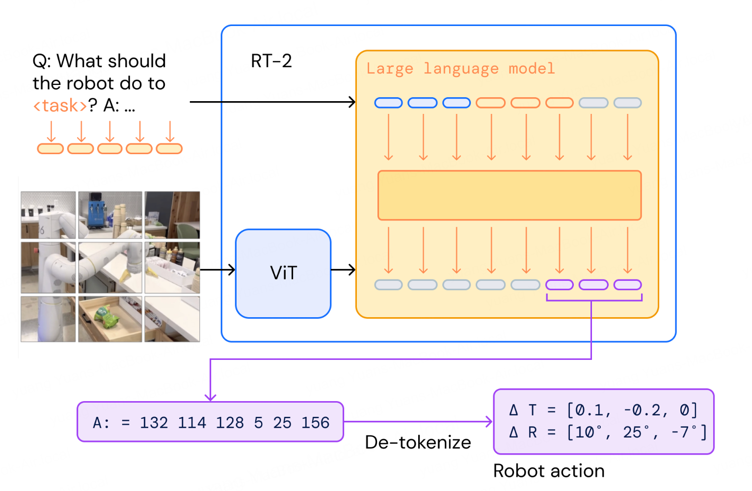
The robotic-transformer paper from google uses a simplified variation of the standard process. It directly represents the robot actions as text strings in a fixed format, so that is still part of the language output, and fine-tuning any VLM is made simple.

\(\pi_0\) Flow Model

\(\pi_0\) model from Physical Intelligence takes another direction: it devised a brand new action tokenization method (FAST) and uses flow-matching diffusion method for action generation.

MLLM (Multimodal Large Language Models)

MLLM systems are trained such that all modalities (vision, audio, text, etc) share the same representational token space. They are modality-agnostic transformers. They use the same principle as VLMs, but generalize it to a broader scope, with video, audio, and image projectors that convert all signals into tokens that LLM can process just like words.

Alignment

This is the extra phase comparing to LLM training, because new modalities need to be projected into text space. The alignment phase is training these other modalities’ projectors with large-scale modal-text pairs. The pre-trained LLM itself is frozen, because the goal is to align embeddings, not teaching LLM new facts.

Instruction Tuning

The LLM weights are then opened and SFT starts, to unlock the reasoning ability. The datasets are usually instructional prompts about answering questions regarding the multi-modal inputs, and LLM is now learning to use its foundational knowledge to reason about those inputs.

RLHF

Similar to LLMs, a preference model or human preference labels with PPO/DPO algorithms extend the RLHF to multimodal inputs.

Beyond Language-Backboned Models

Be it VLM or MLLM, up to now all modalities are projected and unified into word embedding space, where the backbone is a pre-trained LLM that stores foundational knowledge in language domain. This works well in many cases, but we all as human, understand the subtle the linguistic bias of language; text description of the world is a lossy compression—hence the “lost in translation” between languages. Even for a simple image description task, describing every single detail is extremely inefficient. Moreover, human or even animals can perform intuitive spatial reasoning and physics predictions without languages. What if we instead train a model where knowledge is directly stored in “visual token”? This might be one step closer to the ultimate “universal token” that underlies the nature of everything. We can call it the world model.

Storing knowledge in visual token is challenging. The unstructured, continuous nature of vision, and the curse of its high-dimensionality makes tokenizing it just like text extremely hard. There are, however, many works in the specialized realm of robotics that had already made some good attempts: the imaginary rollout by predicting the next frame given current frame and action is already used in some cutting-edge research projects, for example 1X. This new type of simulation enforces the model to internalize fundamental understanding of physics for gravity and object manipulation. This type of vision-based model has however obvious shortcomings: 1. vision captures physics properties such as affordances and dynamics, but they are only physical appearances, lacking the tactile dimension; it’s also unable to capture abstract concepts, which are surprisingly well captured by language, as a compressed form of knowledge; 2. it requires an insane amount of video to train a comprehensive, generalized model that “understands” the dynamics between a variety of scenarios.

NVIDIA Cosmos

Cosmos is a large-scale video-first world foundation model that shifts the backbone of multimodal learning from language to vision and dynamics. Instead of aligning everything into text embedding space, Cosmos learns directly from massive video corpora, storing its foundational knowledge in visual/world tokens.

The training pipeline has three main stages:

• Video tokenization. Raw videos are first compressed into discrete or continuous tokens using specialized video tokenizers (encoder–decoder style, similar to VQ-VAE or neural codecs). This reduces the high-dimensional video space into compact, learnable tokens while retaining spatial–temporal structure.
• World model pre-training. Two model families are trained on hundreds of millions of video clips:
  • Diffusion-based WFMs, which de-noise and predict continuous video tokens.
  • Autoregressive WFMs, which learn to predict future discrete tokens step by step.

  Both approaches push the model to internalize physical dynamics, temporal reasoning, and long-horizon structure beyond static recognition.

• Post-training adaptation. The pretrained WFM is fine-tuned for downstream embodied AI domains:
  • Autonomous driving, where the model predicts future traffic scenes from onboard video.
  • Robotics and manipulation, where it learns affordances and physical causality.
  • 3D navigation and camera control, where the model anticipates environmental changes to guide actions.

To bridge this visual world model with human interaction and higher-level reasoning, Cosmos integrates a language head. World tokens from the video backbone are projected and aligned with text tokens, enabling tasks like instruction following, dialogue, and abstract reasoning. Instruction tuning and RLHF further refine this alignment, so the system can use language as an interface while keeping its foundational knowledge rooted in vision and dynamics.

The key contribution of Cosmos is reframing foundational knowledge as world understanding rather than linguistic reasoning. By learning directly in the video domain, Cosmos aims to capture intuitive physics and causal dynamics that are difficult to compress into language descriptions.

To close the gap between abstract knowledge and symbol grounding, current research usually takes a mixed approach and combine the advantages from both worlds—use language for reasoning and factual knowledge, vision for high-dimensional frame prediction and scene understanding. We are on our way to expand the vision knowledge outside a confined dynamic (e.g., autonomous driving scenarios) and action space (e.g., state space models for robot action planning) to a more generalized, knowledgeable unified MLLM.