Fastest Python Implementation to Find Intersecting Non-Axis-Aligned Convex Polygons
In robotics and autonomous driving, collision checking is an unavoidable topic. For robot arms, the arm-to-world and self-collision checking are crucial for operation safety; for self-driving cars, avoiding collision with other static and dynamic road agents is rather a baseline performance. For robot arm collision checking, the links and joints of the robot arm are often simplified as cylinders and spheres, where fcl library is deployed. More advanced methods such as ray-tracing based collision checking are also applied in certain scenarios. As for the common robot tasks involving grasp, pick-and-place, task planning is heavily dependent on collision checking between target objects and environment constraints. This, together with self-driving car scenarios, can be easily broken down and simplified: project onto 2d plane. In the end, the core utility with high call frequency, is inevitably collision checking between convex polygons.
As a start, we can simplify this problem further: instead of dealing with general polygons, consider the simplest kind, triangles. How to tell if two triangles overlap?

Above are some typical triangle relationships (no pun intended). A naive algorithm would take the vertices of each triangle, compute the edges, and check if any of the edges intersects. We can start from this implementation, but first, we need a very fast way of checking wether two line segments intersect.

We know two line segments \(P_1P_2\) and \(Q_1Q_2\) intersect if and only if:
- Points \(P_1\) and \(P_2\) are on opposite sides of the line formed by segment \(Q_1Q_2\), and
- Points \(Q_1\) and \(Q_2\) are on opposite sides of the line formed by segment \(P_1P_2\).
This means that for the segments to intersect, the endpoints of one segment must “straddle” the line of the other segment, and vice versa. Take the bottom-left case as an example, starting from \(P_1\), the sequence formed by connecting the end points of another segment, \(P_1Q_2Q_1\), differs in the direction from the sequence starting from \(P_2\), \(P_2Q_2Q_1\). Same applies to \(Q\). We can thus quickly determine the intersection, by checking the ordering consistency of sequence pairs: only when the order of \(P_1Q_1Q_2\) is different from that of \(P_2Q_1Q_2\), and \(P_1P_2Q_1\) different from \(P_1P_2Q_2\), are the two segments intersecting. We can thus use cross product to convert the order to signed area, to check if the point sequence is counterclockwise, for fast comparison: if \(AB\times AC > 0\), \(ABC\) is counterclockwise in order.
def ccw(a: np.ndarray, b: np.ndarray, c: np.ndarray) -> bool:
    # Check if (C.y−A.y)⋅(B.x−A.x)−(B.y−A.y)⋅(C.x−A.x) > 0
    return (c[..., 1] - a[..., 1]) * (b[..., 0] - a[..., 0]) > (b[..., 1] - a[..., 1]) * (
        c[..., 0] - a[..., 0]
    )
Note the function is vectorized, written in an extendable way so that arbitrary leading dimensions can be given. This is important for our usage of this function.
Now we can check if two sets of line segments intersect with each other. In the example above, for checking two triangles, we have 1 triangle for each side. If we do not consider the geometric properties, e.g., when two triangles intersect, at least two segments from one side will have intersection, we have three edges each checked three times for another triangle, a total of 9 checks. The simplification from the geometric properties brings no benefits under vectorized computation. Along this thread of thinking, we can extend it easily towards generic polygons. To differentiate the two sides, let’s call one side candidates, and another side judges, so we are checking if each candidate intersects with each judge. The generalized form of judges has shape of \((N, P, 2, D)\), with \(N\) polygons of \(P\) edges, each edge containing 2 end points in \(D=2\) dimensional space. Similarly, the candidates have shape \((M, Q, 2, D)\). To perform the check, we have to namely perform an outer join, so that numpy can broadcast and vectorize the whole computation.
 def check_segment_2d_intersection(
    judges: np.ndarray, candidates: np.ndarray
) -> np.ndarray:
	# judges: N, P, 2, 2; candidates: M, Q, 2, 2
    # Extract coordinates
    p1, p2 = judges[..., 0, :], judges[..., 1, :]  # Shapes: [N, P, 2]
    q1, q2 = candidates[..., 0, :], candidates[..., 1, :]  # Shapes: [M, Q, 2]

    # Expand dimensions for broadcasting
    p1 = p1[..., None, :, None, :]  # Shape: [N, 1, P, 1, 2]
    p2 = p2[..., None, :, None, :]  # Shape: [N, 1, P, 1, 2]
    q1 = q1[None, ..., None, :, :]  # Shape: [1, M, 1, Q, 2]
    q2 = q2[None, ..., None, :, :]  # Shape: [1, M, 1, Q, 2]

    # Check intersections using the ccw function
    cond1 = ccw(p1, q1, q2) != ccw(p2, q1, q2)
    cond2 = ccw(p1, p2, q1) != ccw(p1, p2, q2)
    return cond1 & cond2
With intersection data on line segments, compile this into actual judge vs. candidate results:
result = np.any(segment_itsc_res, axis=(2, 3))
We can now thoroughly test the performance of this method, with varying number of judges and candidates. The benchmark is based on both fixing the number of edges (at 4, for rectangles) with a changing number of candidates and judges, ranging from 1 to 91, and fixing the number of candidates and judges at 40 each, with a changing number of edges, ranging from 3 to 20.
import timeit
from tqdm import tqdm
from matplotlib import pyplot as plt
from functools import partial

# First start with fixed number of edges
def _comp_time_fix_edges():
    t = {}
    i_values = range(1, 101, 10)
    j_values = range(1, 101, 10)
    for i in tqdm(i_values, desc=f'outer loop', position=0):
        x = np.random.random((i, 4, 2, 2))
        t[i] = []
        for j in tqdm(j_values, desc='inner loop', position=1, leave=False):
            p = np.random.random((j, 4, 2, 2))
            t[i].append(timeit.timeit(partial(rectangle_intersection_by_segments, x, p), number=3000) / 3000.)
    return t, i_values, j_values

# Next also fix the number of polygons
def _comp_time_fix_num():
    t = {}
    i_values = range(3, 20, 2)
    j_values = range(3, 20, 2)
    for i in tqdm(i_values, desc=f'outer loop', position=0):
        x = np.random.random((40, i, 2, 2))
        t[i] = []
        for j in tqdm(j_values, desc='inner loop', position=1, leave=False):
            p = np.random.random((40, j, 2, 2))
            t[i].append(timeit.timeit(partial(rectangle_intersection_by_segments, x, p), number=3000) / 3000.)
    return t, i_values, j_values
and with the help of the plotting function,
def plot_timing_data(t: dict, i_values: list, j_values: list, fname: str, fixed_edge: bool):
    # Create a 2D array to store timing data
    timing_data = np.zeros((len(i_values), len(j_values)))

    # Populate the timing data array
    for idx_i, i in enumerate(i_values):
        for idx_j, j in enumerate(j_values):
            timing_data[idx_i, idx_j] = t[i][idx_j]

    # Create a meshgrid for i and j values
    I, J = np.meshgrid(i_values, j_values, indexing='ij')
    fig = plt.figure(figsize=(10, 6))
    ax = fig.add_subplot(111, projection='3d')

    # Plot the surface with transparency
    I_flat = I.flatten()
    J_flat = J.flatten()
    timing_data *= 1000
    timing_flat = timing_data.flatten()

    # Plot the surface with transparency
    surf = ax.plot_surface(I, J, timing_data, cmap='viridis', alpha=0.4, edgecolor='none')

    # Scatter plot (dots)
    scatter = ax.scatter(I_flat, J_flat, timing_flat, c=timing_flat, cmap='viridis', s=10, edgecolor='black')

    # Adjust z-axis limits to capture the actual range of the data
    z_min = np.min(timing_flat)
    z_max = np.max(timing_flat)
    ax.set_zlabel('Time (ms)')
    ax.set_zlim(z_min, z_max)

    if fixed_edge:
        ax.set_xlabel('num_judges (i)')
        ax.set_ylabel('num_candidates (j)')
        ax.set_title('Fixed at 4 edges')
    else:
        ax.set_xlabel('judge_edges (i)')
        ax.set_ylabel('candidate_edges (j)')
        ax.set_title('Fixed at 40 x 40 polygons')

    plt.savefig(f'{fname}.png')
    plt.close()
we get intuitive plots about the performance of the naive algorithm:
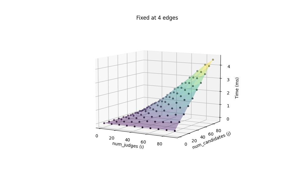
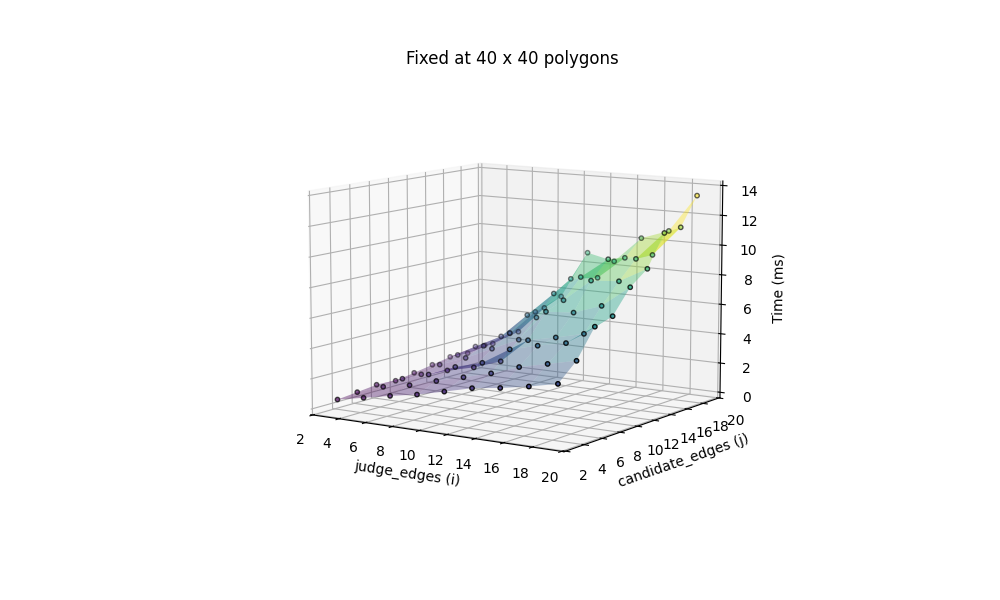
All computation are done on my 2020 M1 MacBook Air. Additionally we include the most challenging situation, with 100 candidates x 100 judges, both icosagons (20 edges), benchmarked at 97.511ms.
The performance seems quite acceptable in this case, but remember, this is a brute force solution, where every single edge pair between candidates and judges are checked. The broadcasted arrays with outer join creates a super high-dimensional blob that consumes enormous amount of memory.
We can still improve the approach, from the opposite side of thinking: if the shapes are not intersecting, that implies there exists a line separating the two. This is the Separating Axis Theorem, which have been explained thoroughly by many blogs. Briefly illustrating the idea here, with courtesy from Newcastle University,
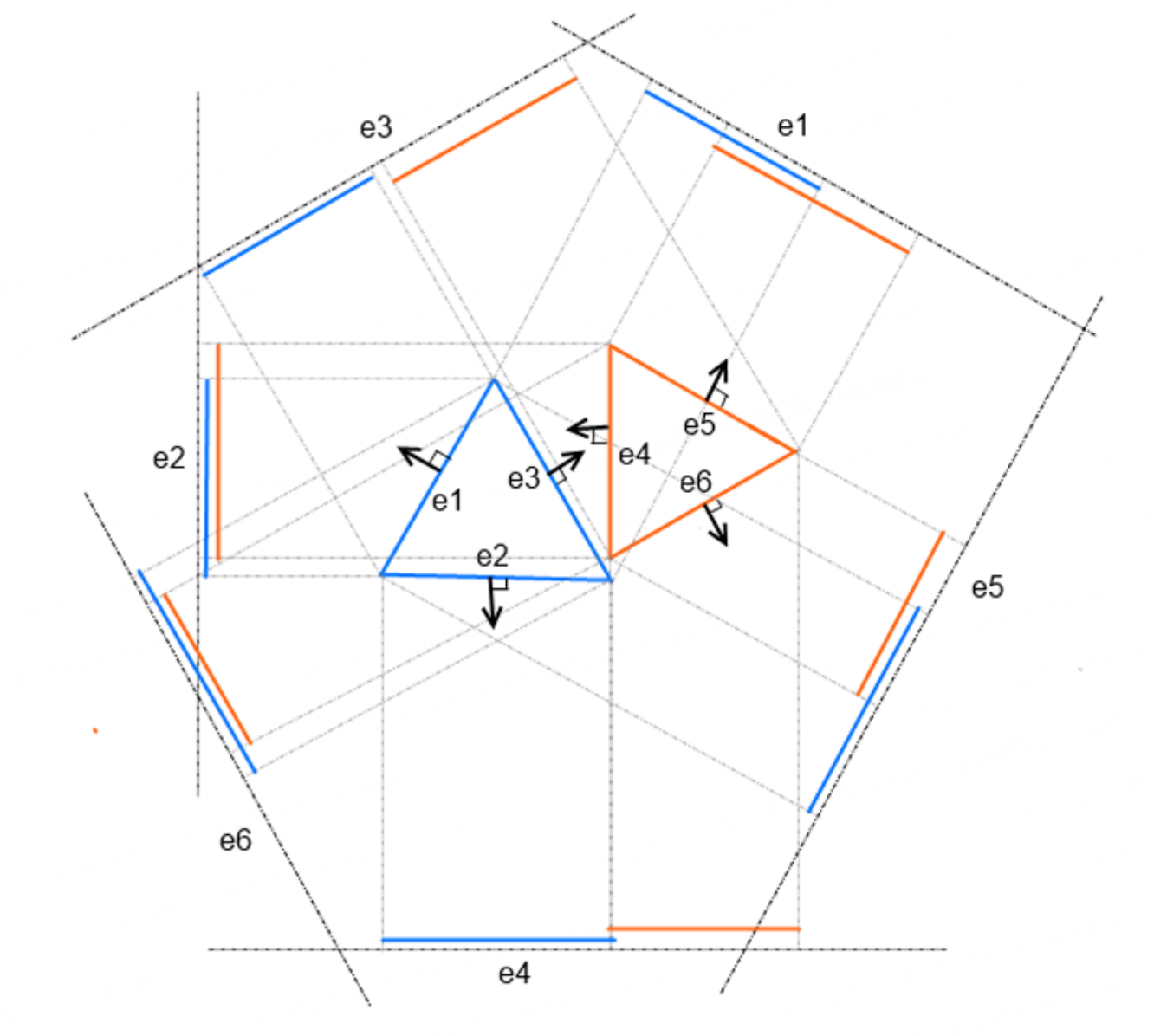
each edge of each polygon is projected to the normals of all edges. The figure above shows 6 projected edges per triangle, because the shorter ones are covered. If there exists any non-overlapping projection, in this case on axis \(e_3\), the polygons are not overlapping. The key difference of this implementation of SAT is vectorized computation. First, we need to define some helper functions to get the edges and their normals:
def vertices_to_edge_vectors(v: np.ndarray) -> np.ndarray:
    """
    Get the edge vectors of the polygons, from their vertices
    """
    return np.roll(v, -1, axis=1) - v

def edge_vectors_to_normal_vectors(e: np.ndarray) -> np.ndarray:
    """
    Get the normal vectors to the edges of the polygons
    """
    assert len(e.shape) == 3
    n = np.empty_like(e)
    n[:, :, 0] = e[:, :, 1]
    n[:, :, 1] = -e[:, :, 0]
    return n / np.expand_dims(np.linalg.norm(n, axis=2), axis=2)
We can then write the fully vectorized version of SAT:
def get_intersecting_polygons(candidates: np.ndarray, judges: np.ndarray) -> np.ndarray:
    """
    Finds which of the |candidates| polygon overlap with the given |judges| polygon.
    Using Separating Axis Theorem (SAT).
    Args:
        candidates: (np.ndarray), N x P x 2
        judges: (np.ndarray), M x P x 2
        where N is number of candidates, M is number of judges, and P is number of vertices
        of the polygon, 2 represents (x, y) 2d plane.
    Returns:
        np.ndarray N x M array indicating whether each candidate intersects with each judge
    """
    candidate_edges = vertices_to_edge_vectors(candidates)
    judge_edges = vertices_to_edge_vectors(judges)

    candidate_normals = edge_vectors_to_normal_vectors(candidate_edges)
    judge_normals = edge_vectors_to_normal_vectors(judge_edges)

    # Compute necessary projections.
    candidate_vertices_on_judge_normals = np.tensordot(candidates, judge_normals.T, axes=1)
    judge_vertices_on_candidate_normals = np.tensordot(judges, candidate_normals.T, axes=1)

    # Compute the projection of each candidate vertex onto each
    # normal vector of its *own* edges, but not those of other candidates. Same
    # for the judges.
    candidate_vertices_on_candidate_normals = np.einsum(
        "ijk,ikm->ijm", candidates, np.transpose(candidate_normals, (0, 2, 1))
    )
    judge_vertices_on_judge_normals = np.einsum(
        "ijk,ikm->ijm", judges, np.transpose(judge_normals, (0, 2, 1))
    )

    judge_vertices_on_judge_normals = np.expand_dims(judge_vertices_on_judge_normals, -1)
    candidate_vertices_on_candidate_normals = np.expand_dims(
        candidate_vertices_on_candidate_normals, -1
    )

    # N x P x 1
    c2c_min = np.min(candidate_vertices_on_candidate_normals, axis=1)
    c2c_max = np.max(candidate_vertices_on_candidate_normals, axis=1)

    # N x P x M
    j2c_min = np.min(judge_vertices_on_candidate_normals, axis=1).T
    j2c_max = np.max(judge_vertices_on_candidate_normals, axis=1).T

    # ==================================================
    # N x P x M
    c2j_min = np.min(candidate_vertices_on_judge_normals, axis=1)
    c2j_max = np.max(candidate_vertices_on_judge_normals, axis=1)

    # 1 x P x M
    j2j_min = np.min(judge_vertices_on_judge_normals, axis=1).T
    j2j_max = np.max(judge_vertices_on_judge_normals, axis=1).T

    # N x P x M, using broadcasting along last axis
    max_endpoint_on_c = np.maximum(c2c_min, j2c_min)
    min_endpoint_on_c = np.minimum(c2c_max, j2c_max)
    projections_overlap_on_candidate_normal = max_endpoint_on_c < min_endpoint_on_c

    # N x P x M, using broadcasting along first axis
    max_endpoint_on_j = np.maximum(c2j_min, j2j_min)
    min_endpoint_on_j = np.minimum(c2j_max, j2j_max)
    projections_overlap_on_judge_normal = max_endpoint_on_j < min_endpoint_on_j

    # N x 2P x M
    projections_overlap = np.concatenate(
        [projections_overlap_on_candidate_normal, projections_overlap_on_judge_normal], axis=1
    )
    # N x M
    return np.all(projections_overlap, axis=1)
Let us also benchmark this implementation:
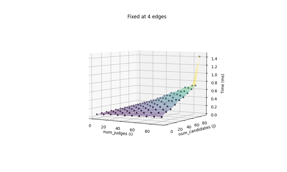
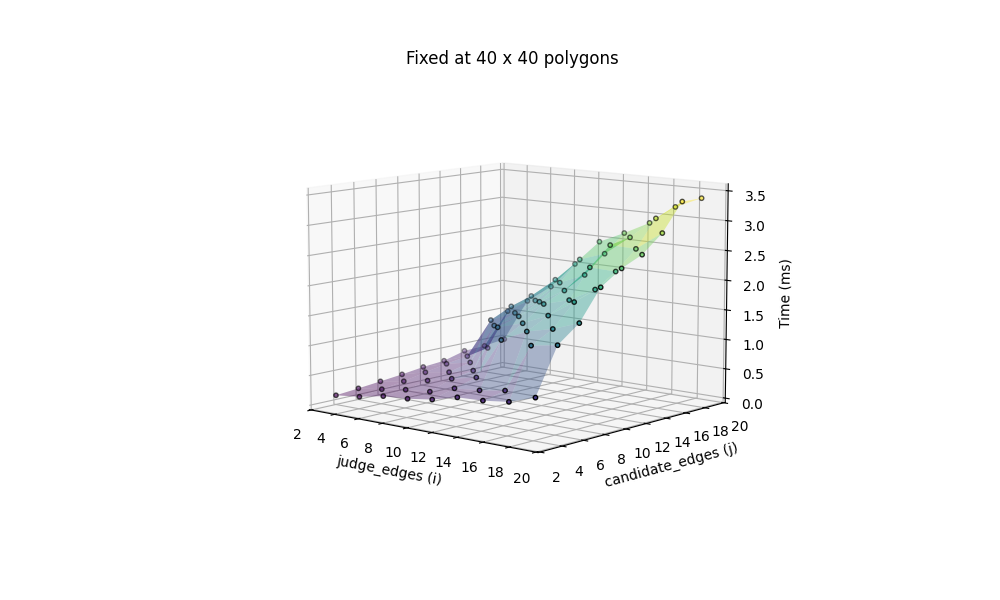
and the same 100 x 100 icosagons takes 22.435ms. This is indeed a 4.4x boost of speed!
One may want to go one step further, so that within candidates or judges, the polygons can have different number of vertices/edges. But wait, before diving into this, why can’t the user first group the polygons by their number of edges and call the intersection checker separately? This mixed shape scenario really brings marginal benefit to actual use cases, so we will skip that. At the end, we may also include a benchmark for the well-known shapely library, but since this is already a very long post, till next time.
Enjoy Reading This Article?
Here are some more articles you might like to read next: